Image: How uncertainty in scientific predictions can help and harm credibility
The Climate Alarm isn’t and was never about the climate, but let’s continue to pretend just so that we can – yet again – falsify the “Green” Rent & Grant Seeking Activists and Criminals and their (FAKE) pseudoscience not everybody understands, including Roy Spencer.
There’s no way to calculate the future cloud cover given we have no way of calculating the sun’s activity and cosmic rays influencing the formation of clouds. The uncertainty is huge and any changes in cloud cover, almost regardless of how small, will have a bigger influence on temperature than CO2 (CO2 has none empirical measured effect to this day).
R. J. L.
By Pat Frank Via WUWT
A bit over a month ago, I posted an essay on WUWT here about my paper assessing the reliability of GCM global air temperature projections in light of error propagation and uncertainty analysis, freely available here.
Four days later, Roy Spencer posted a critique of my analysis at WUWT, here as well as at his own blog, here. The next day, he posted a follow-up critique at WUWT here. He also posted two more critiques on his own blog, here and here.
Curiously, three days before he posted his criticisms of my work, Roy posted an essay, titled, “The Faith Component of Global Warming Predictions,” here. He concluded that, [climate modelers] have only demonstrated what they assumed from the outset. They are guilty of “circular reasoning” and have expressed a “tautology.”
Roy concluded, “I’m not saying that increasing CO₂ doesn’t cause warming. I’m saying we have no idea how much warming it causes because we have no idea what natural energy imbalances exist in the climate system over, say, the last 50 years. … Thus, global warming projections have a large element of faith programmed into them.”
Roy’s conclusion is pretty much a re-statement of the conclusion of my paper, which he then went on to criticize.
In this post, I’ll go through Roy’s criticisms of my work and show why and how every single one of them is wrong.
So, what are Roy’s points of criticism?
He says that:
1) My error propagation predicts huge excursions of temperature.
2) Climate Models Do NOT Have Substantial Errors in their TOA Net Energy Flux
3) The Error Propagation Model is Not Appropriate for Climate Models
I’ll take these in turn.
This is a long post. For those wishing just the executive summary, all of Roy’s criticisms are badly misconceived.
1) Error propagation predicts huge excursions of temperature.
Roy wrote, “Frank’s paper takes an example known bias in a typical climate model’s longwave (infrared) cloud forcing (LWCF) and assumes that the typical model’s error (+/-4 W/m2) in LWCF can be applied in his emulation model equation, propagating the error forward in time during his emulation model’s integration. The result is a huge (as much as 20 deg. C or more) of resulting spurious model warming (or cooling) in future global average surface air temperature (GASAT). (my bold)”
For the attention of Mr. And then There’s Physics, and others, Roy went on to write this: “The modelers are well aware of these biases [in cloud fraction], which can be positive or negative depending upon the model. The errors show that (for example) we do not understand clouds and all of the processes controlling their formation and dissipation from basic first physical principles, otherwise all models would get very nearly the same cloud amounts.” No more dismissals of root-mean-square error, please.
Here is Roy’s Figure 1, demonstrating his first major mistake. I’ve bolded the evidential wording.
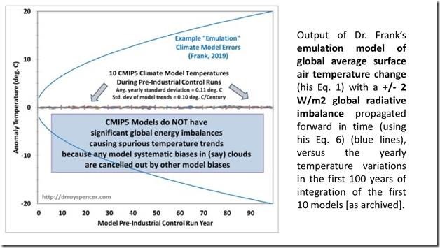
Roy’s blue lines are not air temperatures emulated using equation 1 from the paper. They do not come from eqn. 1, and do not represent physical air temperatures at all.
They come from eqns. 5 and 6, and are the growing uncertainty bounds in projected air temperatures. Uncertainty statistics are not physical temperatures.
Roy misconceived his ±2 Wm-2 as a radiative imbalance. In the proper context of my analysis, it should be seen as a ±2 Wm-2 uncertainty in long wave cloud forcing (LWCF). It is a statistic, not an energy flux.
Even worse, were we to take Roy’s ±2 Wm-2 to be a radiative imbalance in a model simulation; one that results in an excursion in simulated air temperature, (which is Roy’s meaning), we then have to suppose the imbalance is both positive and negative at the same time, i.e., ±radiative forcing.
A ±radiative forcing does not alternate between +radiative forcing and -radiative forcing. Rather it is both signs together at once.
So, Roy’s interpretation of LWCF ±error as an imbalance in radiative forcing requires simultaneous positive and negative temperatures.
Look at Roy’s Figure. He represents the emulated air temperature to be a hot house and an ice house simultaneously; both +20 C and -20 C coexist after 100 years. That is the nonsensical message of Roy’s blue lines, if we are to assign his meaning that the ±2 Wm-2 is radiative imbalance.
That physically impossible meaning should have been a give-away that the basic supposition was wrong.
The ± is not, after all, one or the other, plus or minus. It is coincidental plus and minus, because it is part of a root-mean-square-error (rmse) uncertainty statistic. It is not attached to a physical energy flux.
It’s truly curious. More than one of my reviewers made the same very naive mistake that ±C = physically real +C or -C. This one, for example, which is quoted in the Supporting Information: “The author’s error propagation is not] physically justifiable. (For instance, even after forcings have stabilized, [the author’s] analysis would predict that the models will swing ever more wildly between snowball and runaway greenhouse states. Which, it should be obvious, does not actually happen).“
Any understanding of uncertainty analysis is clearly missing.
Likewise, this first part of Roy’s point 1 is completely misconceived.
Next mistake in the first criticism: Roy says that the emulation equation does not yield the flat GCM control run line in his Figure 1.
However, emulation equation 1 would indeed give the same flat line as the GCM control runs under zero external forcing. As proof, here’s equation 1:

In a control run there is no change in forcing, so DFi = 0. The fraction in the brackets then becomes F0/F0 = 1.
The originating fCO₂ = 0.42 so that equation 1 becomes, DTi(K) = 0.42´33K´1 + a = 13.9 C +a = constant (a = 273.1 K or 0 C).
When an anomaly is taken, the emulated temperature change is constant zero, just as in Roy’s GCM control runs in Figure 1.
So, Roy’s first objection demonstrates three mistakes.
1) Roy mistakes a rms statistical uncertainty in simulated LWCF as a physical radiative imbalance.
2) He then mistakes a ±uncertainty in air temperature as a physical temperature.
3) His analysis of emulation equation 1 was careless.
Next, Roy’s 2): Climate Models Do NOT Have Substantial Errors in their TOA Net Energy Flux
Roy wrote, “If any climate model has as large as a 4 W/m2 bias in top-of-atmosphere (TOA) energy flux, it would cause substantial spurious warming or cooling. None of them do.”
I will now show why this objection is irrelevant.
Here, now, is Roy’s second figure, again showing the perfect TOA radiative balance of CMIP5 climate models. On the right, next to Roy’s figure, is Figure 4 from the paper showing the total cloud fraction (TCF) annual error of 12 CMIP5 climate models, averaging ±12.1%. [1]
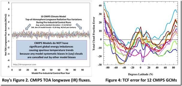
Every single one of the CMIP5 models that produced average ±12.1% of simulated total cloud fraction error also featured Roy’s perfect TOA radiative balance.
Therefore, every single CMIP5 model that averaged ±4 Wm-2 in LWCF error also featured Roy’s perfect TOA radiative balance.
How is that possible? How can models maintain perfect simulated TOA balance while at the same time producing errors in long wave cloud forcing?
Off-setting errors, that’s how. GCMs are required to have TOA balance. So, parameters are adjusted within their uncertainty bounds so as to obtain that result.
Roy says so himself: “If a model has been forced to be in global energy balance, then energy flux component biases have been cancelled out, …”
Are the chosen GCM parameter values physically correct? No one knows.
Are the parameter sets identical model-to-model? No. We know that because different models produce different profiles and integrated intensities of TCF error.
This removes all force from Roy’s TOA objection. Models show TOA balance and LWCF error simultaneously.
In any case, this goes to the point raised earlier, and in the paper, that a simulated climate can be perfectly in TOA balance while the simulated climate internal energy state is incorrect.
That means that the physics describing the simulated climate state is incorrect. This in turn means that the physics describing the simulated air temperature is incorrect.
The simulated air temperature is not grounded in physical knowledge. And that means there is a large uncertainty in projected air temperature because we have no good physically causal explanation for it.
The physics can’t describe it; the model can’t resolve it. The apparent certainty in projected air temperature is a chimerical result of tuning.
This is the crux idea of an uncertainty analysis. One can get the observables right. But if the wrong physics gives the right answer, one has learned nothing and one understands nothing. The uncertainty in the result is consequently large.
This wrong physics is present in every single step of a climate simulation. The calculated air temperatures are not grounded in a physically correct theory.
Roy says the LWCF error is unimportant because all the errors cancel out. I’ll get to that point below. But notice what he’s saying: the wrong physics allows the right answer. And invariably so in every step all the way across a 100-year projection.
In his September 12 criticism, Roy gives his reason for disbelief in uncertainty analysis: “All of the models show the effect of anthropogenic CO2 emissions, despite known errors in components of their energy fluxes (such as clouds)!
“Why?
“If a model has been forced to be in global energy balance, then energy flux component biases have been cancelled out, as evidenced by the control runs of the various climate models in their LW (longwave infrared) behavior.”
There it is: wrong physics that is invariably correct in every step all the way across a 100-year projection, because large-scale errors cancel to reveal the effects of tiny perturbations. I don’t believe any other branch of physical science would countenance such a claim.
Roy then again presented the TOA radiative simulations on the left of the second set of figures above.
Roy wrote that models are forced into TOA balance. That means the physical errors that might have appeared as TOA imbalances are force-distributed into the simulated climate sub-states.
Forcing models to be in TOA balance may even make simulated climate subsystems more in error than they would otherwise be.
After observing that the “forced-balancing of the global energy budget“ is done only once for the “multi-century pre-industrial control runs,” Roy observed that models world-wide behave similarly despite a, “WIDE variety of errors in the component energy fluxes…”
Roy’s is an interesting statement, given there is nearly a factor of three difference among models in their sensitivity to doubled CO₂. [2, 3]
According to Stephens [3], “This discrepancy is widely believed to be due to uncertainties in cloud feedbacks. … Fig. 1 [shows] the changes in low clouds predicted by two versions of models that lie at either end of the range of warming responses. The reduced warming predicted by one model is a consequence of increased low cloudiness in that model whereas the enhanced warming of the other model can be traced to decreased low cloudiness. (original emphasis)”
So, two CMIP5 models show opposite trends in simulated cloud fraction in response to CO₂ forcing. Nevertheless, they both reproduce the historical trend in air temperature.
Not only that, but they’re supposedly invariably correct in every step all the way across a 100-year projection, because their large-scale errors cancel to reveal the effects of tiny perturbations.
In Stephen’s object example we can see the hidden simulation uncertainty made manifest. Models reproduce calibration observables by hook or by crook, and then on those grounds are touted as able to accurately predict future climate states.
The Stephens example provides clear evidence that GCMs plain cannot resolve the cloud response to CO₂ emissions. Therefore, GCMs cannot resolve the change in air temperature, if any, from CO₂ emissions. Their projected air temperatures are not known to be physically correct. They are not known to have physical meaning.
This is the reason for the large and increasing step-wise simulation uncertainty in projected air temperature.
This obviates Roy’s point about cancelling errors. The models cannot resolve the cloud response to CO₂ forcing. Cancellation of radiative forcing errors does not repair this problem. Such cancellation (from by-hand tuning) just speciously hides the simulation uncertainty.
Roy concluded that, “Thus, the models themselves demonstrate that their global warming forecasts do not depend upon those bias errors in the components of the energy fluxes (such as global cloud cover) as claimed by Dr. Frank (above).“I
Everyone should now know why Roy’s view is wrong. Off-setting errors make models similar to one another. They do not make the models accurate. Nor do they improve the physical description.
Roy’s conclusion implicitly reveals his mistaken thinking.
1) The inability of GCMs to resolve cloud response means the temperature projection consistency among models is a chimerical artifact of their tuning. The uncertainty remains in the projection; it’s just hidden from view.
2) The LWCF ±4 Wm-2 rmse is not a constant offset bias error. The ‘±’ alone should be enough to tell anyone that it does not represent an energy flux.
The LWCF ±4 Wm-2 rmse represents an uncertainty in simulated energy flux. It’s not a physical error at all.
One can tune the model to produce (simulation minus observation = 0) no observable error at all in their calibration period. But the physics underlying the simulation is wrong. The causality is not revealed. The simulation conveys no information. The result is not any indicator of physical accuracy. The uncertainty is not dismissed.
3) All the models making those errors are forced to be in TOA balance. Those TOA-balanced CMIP5 models make errors averaging ±12.1% in global TCF.[1] This means the GCMs cannot model cloud cover to better resolution than ±12.1%.
To minimally resolve the effect of annual CO₂ emissions, they need to be at about 0.1% cloud resolution (see Appendix 1 below)
4) The average GCM error in simulated TCF over the calibration hindcast time reveals the average calibration error in simulated long wave cloud forcing. Even though TOA balance is maintained throughout, the correct magnitude of simulated tropospheric thermal energy flux is lost within an uncertainty interval of ±4 Wm-2.
Roy’s 3) Propagation of error is inappropriate.
On his blog, Roy wrote that modeling the climate is like modeling pots of boiling water. Thus, “[If our model] can get a constant water temperature, [we know] that those rates of energy gain and energy loss are equal, even though we don’t know their values. And that, if we run [the model] with a little more coverage of the pot by the lid, we know the modeled water temperature will increase. That part of the physics is still in the model.”
Roy continued, “the temperature change in anything, including the climate system, is due to an imbalance between energy gain and energy loss by the system.”
Roy there implied that the only way air temperature can change is by way of an increase or decrease of the total energy in the climate system. However, that is not correct.
Climate subsystems can exchange energy. Air temperature can change by redistribution of internal energy flux without any change in the total energy entering or leaving the climate system.
For example, in his 2001 testimony before the Senate Environment and Public Works Committee on 2 May, Richard Lindzen noted that, “claims that man has contributed any of the observed warming (ie attribution) are based on the assumption that models correctly predict natural variability. [However,] natural variability does not require any external forcing – natural or anthropogenic. (my bold)” [4]
Richard Lindzen noted exactly the same thing in his, “Some Coolness Concerning Global Warming. [5]
“The precise origin of natural variability is still uncertain, but it is not that surprising. Although the solar energy received by the earth-ocean-atmosphere system is relatively constant, the degree to which this energy is stored and released by the oceans is not. As a result, the energy available to the atmosphere alone is also not constant. … Indeed, our climate has been both warmer and colder than at present, due solely to the natural variability of the system. External influences are hardly required for such variability to occur.(my bold)”
In his review of Stephen Schneider’s “Laboratory Earth,” [6] Richard Lindzen wrote this directly relevant observation,
“A doubling CO₂ in the atmosphere results in a two percent perturbation to the atmosphere’s energy balance. But the models used to predict the atmosphere’s response to this perturbation have errors on the order of ten percent in their representation of the energy balance, and these errors involve, among other things, the feedbacks which are crucial to the resulting calculations. Thus the models are of little use in assessing the climatic response to such delicate disturbances. Further, the large responses (corresponding to high sensitivity) of models to the small perturbation that would result from a doubling of carbon dioxide crucially depend on positive (or amplifying) feedbacks from processes demonstrably misrepresented by models. (my bold)”
These observations alone are sufficient to refute Roy’s description of modeling air temperature in analogy to the heat entering and leaving a pot of boiling water with varying amounts of lid-cover.
Richard Lindzen’s last point, especially, contradicts Roy’s claim that cancelling simulation errors permit a reliably modeled response to forcing or accurately projected air temperatures.
Also, the situation is much more complex than Roy described in his boiling pot analogy. For example, rather than Roy’s single lid moving about, clouds are more like multiple layers of sieve-like lids of varying mesh size and thickness, all in constant motion, and none of them covering the entire pot.
The pot-modeling then proceeds with only a poor notion of where the various lids are at any given time, and without fully understanding their depth or porosity.
Propagation of error: Given an annual average +0.035 Wm-2 increase in CO₂ forcing, the increase plus uncertainty in the simulated tropospheric thermal energy flux is (0.035±4) Wm-2. All the while simulated TOA balance is maintained.
So, if one wanted to calculate the uncertainty interval for the air temperature for any specific annual step, the top of the temperature uncertainty interval would be calculated from +4.035 Wm-2, while the bottom of the interval would be -3.9065 Wm-2.
Putting that into the right side of paper eqn. 5.2 and setting F0=33.30 Wm-2, then the single-step projection uncertainty interval in simulated air temperature is +1.68 C/-1.63 C.
The air temperature anomaly projected from the average CMIP5 GCM would, however, be 0.015 C; not +1.68 C or -1.63 C.
In the whole modeling exercise, the simulated TOA balance is maintained. Simulated TOA balance is maintained mainly because simulation error in long wave cloud forcing is offset by simulation error in short wave cloud forcing.
This means the underlying physics is wrong and the simulated climate energy state is wrong. Over the calibration hindcast region, the observed air temperature is correctly reproduced only because of curve fitting following from the by-hand adjustment of model parameters.[2, 7]
Forced correspondence with a known value does not remove uncertainty in a result, because causal ignorance is unresolved.
When error in an intermediate result is imposed on every single step of a sequential series of calculations — which describes an air temperature projection — that error gets transmitted into the next step. The next step adds its own error onto the top of the prior level. The only way to gauge the effect of step-wise imposed error is step-wise propagation of the appropriate rmse uncertainty.
Figure 3 below shows the problem in a graphical way. GCMs project temperature in a step-wise sequence of calculations. [8] Incorrect physics means each step is in error. The climate energy-state is wrong (this diagnosis also applies to the equilibrated base state climate).
The wrong climate state gets calculationally stepped forward. Its error constitutes the initial conditions of the next step. Incorrect physics means the next step produces its own errors. Those new errors add onto the entering initial condition errors. And so it goes, step-by-step. The errors add with every step.
When one is calculating a future state, one does not know the sign or magnitude of any of the errors in the result. This ignorance follows from the obvious difficulty that there are no observations available from a future climate.
The reliability of the projection then must be judged from an uncertainty analysis. One calibrates the model against known observables (e.g., total cloud fraction). By this means, one obtains a relevant estimate of model accuracy; an appropriate average root-mean-square calibration error statistic.
The calibration error statistic informs us of the accuracy of each calculational step of a simulation. When inaccuracy is present in each step, propagation of the calibration error metric is carried out through each step. Doing so reveals the uncertainty in the result — how much confidence we should put in the number.
When the calculation involves multiple sequential steps each of which transmits its own error, then the step-wise uncertainty statistic is propagated through the sequence of steps. The uncertainty of the result must grow. This circumstance is illustrated in Figure 3.
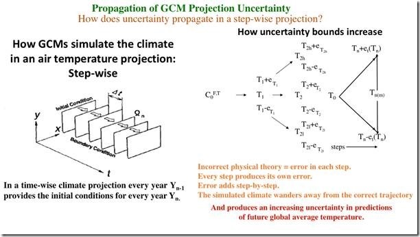
Figure 3: Growth of uncertainty in an air temperature projection. ![]() is the base state climate that has an initial forcing, F0, which may be zero, and an initial temperature, T0. The final temperature Tn is conditioned by the final uncertainty ±et, as Tn±et.
is the base state climate that has an initial forcing, F0, which may be zero, and an initial temperature, T0. The final temperature Tn is conditioned by the final uncertainty ±et, as Tn±et.
Step one projects a first-step forcing F1, which produces a temperature T1. Incorrect physics introduces a physical error in temperature, e1, which may be positive or negative. In a projection of future climate, we do not know the sign or magnitude of e1.
However, hindcast calibration experiments tell us that single projection steps have an average uncertainty of ±e.
T1 therefore has an uncertainty of ![]()
The step one temperature plus its physical error, T1+e1, enters step 2 as its initial condition. But T1 had an error, e1. That e1 is an error offset of unknown sign in T1. Therefore, the incorrect physics of step 2 receives a T1 that is offset by e1. But in a futures-projection, one does not know the value of T1+e1.
In step 2, incorrect physics starts with the incorrect T1 and imposes new unknown physical error e2 on T2. The error in T2 is now e1+e2. However, in a futures-projection the sign and magnitude of e1, e2 and their sum remain unknown.
And so it goes; step 3, …, n add in their errors e3 +, …, + en. But in the absence of knowledge concerning the sign or magnitude of the imposed errors, we do not know the total error in the final state. All we do know is that the trajectory of the simulated climate has wandered away from the trajectory of the physically correct climate.
However, the calibration error statistic provides an estimate of the uncertainty in the results of any single calculational step, which is ±e.
When there are multiple calculational steps, ±e attaches independently to every step. The predictive uncertainty increases with every step because the ±e uncertainty gets propagated through those steps to reflect the continuous but unknown impact of error. Propagation of calibration uncertainty goes as the root-sum-square (rss). For ‘n’ steps that’s ![]() . [9-11]
. [9-11]
It should be very clear to everyone that the rss equation does not produce physical temperatures, or the physical magnitudes of anything else. it is a statistic of predictive uncertainty that necessarily increases with the number of calculational steps in the prediction. A summary of the uncertainty literature was commented into my original post, here.
The growth of uncertainty does not mean the projected air temperature becomes huge. Projected temperature is always within some physical bound. But the reliability of that temperature — our confidence that it is physically correct — diminishes with each step. The level of confidence is the meaning of uncertainty. As confidence diminishes, uncertainty grows.
Supporting Information Section 10.2 discusses uncertainty and its meaning. C. Roy and J. Oberkampf (2011) describe it this way, “[predictive] uncertainty [is] due to lack of knowledge by the modelers, analysts conducting the analysis, or experimentalists involved in validation. The lack of knowledge can pertain to, for example, modeling of the system of interest or its surroundings, simulation aspects such as numerical solution error and computer roundoff error, and lack of experimental data.” [12]
The growth of uncertainty means that with each step we have less and less knowledge of where the simulated future climate is, relative to the physically correct future climate. Figure 3 shows the widening scope of uncertainty with the number of steps.
Wide uncertainty bounds mean the projected temperature reflects a future climate state that is some completely unknown distance from the physically real future climate state. One’s confidence is minimal that the simulated future temperature is the ‘true’ future temperature.
This is why propagation of uncertainty through an air temperature projection is entirely appropriate. It is our only estimate of the reliability of a predictive result.
Appendix 1 below shows that the models need to simulate clouds to about ±0.1% accuracy, about 100 times better than ±12.1% the they now do, in order to resolve any possible effect of CO₂ forcing.
Appendix 2 quotes Richard Lindzen on the utter corruption and dishonesty that pervades AGW consensus climatology.
Before proceeding, here’s NASA on clouds and resolution: “A doubling in atmospheric carbon dioxide (CO2), predicted to take place in the next 50 to 100 years, is expected to change the radiation balance at the surface by only about 2 percent. … If a 2 percent change is that important, then a climate model to be useful must be accurate to something like 0.25%. Thus today’s models must be improved by about a hundredfold in accuracy, a very challenging task.”
That hundred-fold is exactly the message of my paper.
If climate models cannot resolve the response of clouds to CO₂ emissions, they can’t possibly accurately project the impact of CO₂ emission on air temperature?
The ±4 Wm-2 uncertainty in LWCF is a direct reflection of the profound ignorance surrounding cloud response.
The CMIP5 LWCF calibration uncertainty reflects ignorance concerning the magnitude of the thermal flux in the simulated troposphere that is a direct consequence of the poor ability of CMIP5 models to simulate cloud fraction.
From page 9 in the paper, “This climate model error represents a range of atmospheric energy flux uncertainty within which smaller energetic effects cannot be resolved within any CMIP5 simulation.”
The 0.035 Wm-2 annual average CO₂ forcing is exactly such a smaller energetic effect.
It is impossible to resolve the effect on air temperature of a 0.035 Wm-2 change in forcing, when the model cannot resolve overall tropospheric forcing to better than ±4 Wm-2.
The perturbation is ±114 times smaller than the lower limit of resolution of a CMIP5 GCM.
The uncertainty interval can be appropriately analogized as the smallest simulation pixel size. It is the blur level. It is the ignorance width within which nothing is known.
Uncertainty is not a physical error. It does not subtract away. It is a measure of ignorance.
The model can produce a number. When the physical uncertainty is large, that number is physically meaningless.
All of this is discussed in the paper, and in exhaustive detail in Section 10 of the Supporting Information. It’s not as though that analysis is missing or cryptic. It is pretty much invariably un-consulted by my critics, however.
Smaller strange and mistaken ideas:
Roy wrote, “If a model actually had a +4 W/m2 imbalance in the TOA energy fluxes, that bias would remain relatively constant over time.”
But the LWCF error statistic is ±4 Wm-2, not (+)4 Wm-2 imbalance in radiative flux. Here, Roy has not only misconceived a calibration error statistic as an energy flux, but has facilitated the mistaken idea by converting the ± into (+).
This mistake is also common among my prior reviewers. It allowed them to assume a constant offset error. That in turn allowed them to assert that all error subtracts away.
This assumption of perfection after subtraction is a folk-belief among consensus climatologists. It is refuted right in front of their eyes by their own results, (Figure 1 in [13]) but that never seems to matter.
Another example includes Figure 1 in the paper, which shows simulated temperature anomalies. They are all produced by subtracting away a simulated climate base-state temperature. If the simulation errors subtracted away, all the anomaly trends would be superimposed. But they’re far from that ideal.
Figure 4 shows a CMIP5 example of the same refutation.
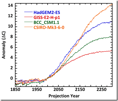
Figure 4: RCP8.5 projections from four CMIP5 models.
Model tuning has made all four projection anomaly trends close to agreement from 1850 through 2000. However, after that the models career off on separate temperature paths. By projection year 2300, they range across 8 C. The anomaly trends are not superimposable; the simulation errors have not subtracted away.
The idea that errors subtract away in anomalies is objectively wrong. The uncertainties that are hidden in the projections after year 2000, by the way, are also in the projections from 1850-2000 as well.
This is because the projections of the historical temperatures rest on the same wrong physics as the futures projection. Even though the observables are reproduced, the physical causality underlying the temperature trend is only poorly described in the model. Total cloud fraction is just as wrongly simulated for 1950 as it is for 2050.
LWCF error is present throughout the simulations. The average annual ±4 Wm-2 simulation uncertainty in tropospheric thermal energy flux is present throughout, putting uncertainty into every simulation step of air temperature. Tuning the model to reproduce the observables merely hides the uncertainty.
Roy wrote, “Another curious aspect of Eq. 6 is that it will produce wildly different results depending upon the length of the assumed time step.”
But, of course, eqn. 6 would not produce wildly different results because simulation error varies with the length of the GCM time step.
For example, we can estimate the average per-day uncertainty from the ±4 Wm-2 annual average calibration of Lauer and Hamilton.
So, for the entire year (±4 Wm–2)2 = ![]() , where ei is the per-day uncertainty. This equation yields, ei = ±0.21 Wm–2 for the estimated LWCF uncertainty per average projection day. If we put the daily estimate into the right side of equation 5.2 in the paper and set F0=33.30 Wm-2, then the one-day per-step uncertainty in projected air temperature is ±0.087 C. The total uncertainty after 100 years is sqrt[(0.087)2´365´100] = ±16.6 C.
, where ei is the per-day uncertainty. This equation yields, ei = ±0.21 Wm–2 for the estimated LWCF uncertainty per average projection day. If we put the daily estimate into the right side of equation 5.2 in the paper and set F0=33.30 Wm-2, then the one-day per-step uncertainty in projected air temperature is ±0.087 C. The total uncertainty after 100 years is sqrt[(0.087)2´365´100] = ±16.6 C.
The same approach yields an estimated 25-year mean model calibration uncertainty to be sqrt[(±4 Wm–2)2´25] = ±20 Wm–2. Following from eqn. 5.2, the 25-year per-step uncertainty is ±8.3 C. After 100 years the uncertainty in projected air temperature is sqrt[(±8.3)2´4)] = ±16.6 C.
Roy finished with, “I’d be glad to be proved wrong.”
Be glad, Roy.
Appendix 1: Why CMIP5 error in TCF is important.
We know from Lauer and Hamilton that the average CMIP5 ±12.1% annual total cloud fraction (TCF) error produces an annual average ±4 Wm-2 calibration error in long wave cloud forcing. [14]
We also know that the annual average increase in CO₂ forcing since 1979 is about 0.035 Wm-2 (my calculation).
Assuming a linear relationship between cloud fraction error and LWCF error, the ±12.1% CF error is proportionately responsible for ±4 Wm-2 annual average LWCF error.
Then one can estimate the level of resolution necessary to reveal the annual average cloud fraction response to CO₂ forcing as:
[(0.035 Wm-2/±4 Wm-2)]*±12.1% total cloud fraction = 0.11% change in cloud fraction.
This indicates that a climate model needs to be able to accurately simulate a 0.11% feedback response in cloud fraction to barely resolve the annual impact of CO₂ emissions on the climate. If one wants accurate simulation, the model resolution should be ten times small than the effect to be resolved. That means 0.011% accuracy in simulating annual average TCF.
That is, the cloud feedback to a 0.035 Wm-2 annual CO₂ forcing needs to be known, and able to be simulated, to a resolution of 0.11% in TCF in order to minimally know how clouds respond to annual CO₂ forcing.
Here’s an alternative way to get at the same information. We know the total tropospheric cloud feedback effect is about -25 Wm-2. [15] This is the cumulative influence of 67% global cloud fraction.
The annual tropospheric CO₂ forcing is, again, about 0.035 Wm-2. The CF equivalent that produces this feedback energy flux is again linearly estimated as (0.035 Wm-2/25 Wm-2)*67% = 0.094%. That’s again bare-bones simulation. Accurate simulation requires ten times finer resolution, which is 0.0094% of average annual TCF.
Assuming the linear relations are reasonable, both methods indicate that the minimal model resolution needed to accurately simulate the annual cloud feedback response of the climate, to an annual 0.035 Wm-2 of CO₂ forcing, is about 0.1% CF.
To achieve that level of resolution, the model must accurately simulate cloud type, cloud distribution and cloud height, as well as precipitation and tropical thunderstorms.
This analysis illustrates the meaning of the annual average ±4 Wm-2 LWCF error. That error indicates the overall level of ignorance concerning cloud response and feedback.
The TCF ignorance is such that the annual average tropospheric thermal energy flux is never known to better than ±4 Wm-2. This is true whether forcing from CO₂ emissions is present or not.
This is true in an equilibrated base-state climate as well. Running a model for 500 projection years does not repair broken physics.
GCMs cannot simulate cloud response to 0.1% annual accuracy. It is not possible to simulate how clouds will respond to CO₂ forcing.
It is therefore not possible to simulate the effect of CO₂ emissions, if any, on air temperature.
As the model steps through the projection, our knowledge of the consequent global air temperature steadily diminishes because a GCM cannot accurately simulate the global cloud response to CO₂ forcing, and thus cloud feedback, at all for any step.
It is true in every step of a simulation. And it means that projection uncertainty compounds because every erroneous intermediate climate state is subjected to further simulation error.
This is why the uncertainty in projected air temperature increases so dramatically. The model is step-by-step walking away from initial value knowledge, further and further into ignorance.
On an annual average basis, the uncertainty in CF feedback is ±144 times larger than the perturbation to be resolved.
The CF response is so poorly known, that even the first simulation step enters terra incognita.
Appendix 2: On the Corruption and Dishonesty in Consensus Climatology
It is worth quoting Lindzen on the effects of a politicized science. [16]”A second aspect of politicization of discourse specifically involves scientific literature. Articles challenging the claim of alarming response to anthropogenic greenhouse gases are met with unusually quick rebuttals. These rebuttals are usually published as independent papers rather than as correspondence concerning the original articles, the latter being the usual practice. When the usual practice is used, then the response of the original author(s) is published side by side with the critique. However, in the present situation, such responses are delayed by as much as a year. In my experience, criticisms do not reflect a good understanding of the original work. When the original authors’ responses finally appear, they are accompanied by another rebuttal that generally ignores the responses but repeats the criticism. This is clearly not a process conducive to scientific progress, but it is not clear that progress is what is desired. Rather, the mere existence of criticism entitles the environmental press to refer to the original result as ‘discredited,’ while the long delay of the response by the original authors permits these responses to be totally ignored.
“A final aspect of politicization is the explicit intimidation of scientists. Intimidation has mostly, but not exclusively, been used against those questioning alarmism. Victims of such intimidation generally remain silent. Congressional hearings have been used to pressure scientists who question the ‘consensus’. Scientists who views question alarm are pitted against carefully selected opponents. The clear intent is to discredit the ‘skeptical’ scientist from whom a ‘recantation’ is sought.“[7]
Richard Lindzen’s extraordinary account of the jungle of dishonesty that is consensus climatology is required reading. None of the academics he names as participants in chicanery deserve continued employment as scientists. [16]
If one tracks his comments from the earliest days to near the present, his growing disenfranchisement becomes painful and obvious.[4-7, 16, 17] His “Climate Science: Is it Currently Designed to Answer Questions?” is worth reading in its entirety.
References:
[1] Jiang, J.H., et al., Evaluation of cloud and water vapor simulations in CMIP5 climate models using NASA “A-Train” satellite observations. J. Geophys. Res., 2012. 117(D14): p. D14105.
[2] Kiehl, J.T., Twentieth century climate model response and climate sensitivity. Geophys. Res. Lett., 2007. 34(22): p. L22710.
[3] Stephens, G.L., Cloud Feedbacks in the Climate System: A Critical Review. J. Climate, 2005. 18(2): p. 237-273.
[4] Lindzen, R.S. (2001) Testimony of Richard S. Lindzen before the Senate Environment and Public Works Committee on 2 May 2001. URL: http://www-eaps.mit.edu/faculty/lindzen/Testimony/Senate2001.pdf Date Accessed:
[5] Lindzen, R., Some Coolness Concerning Warming. BAMS, 1990. 71(3): p. 288-299.
[6] Lindzen, R.S. (1998) Review of Laboratory Earth: The Planetary Gamble We Can’t Afford to Lose by Stephen H. Schneider (New York: Basic Books, 1997) 174 pages. Regulation, 5 URL: https://www.cato.org/sites/cato.org/files/serials/files/regulation/1998/4/read2-98.pdf Date Accessed: 12 October 2019.
[7] Lindzen, R.S., Is there a basis for global warming alarm?, in Global Warming: Looking Beyond Kyoto, E. Zedillo ed, 2006 in Press The full text is available at: https://ycsg.yale.edu/assets/downloads/kyoto/LindzenYaleMtg.pdf Last accessed: 12 October 2019, Yale University: New Haven.
[8] Saitoh, T.S. and S. Wakashima, An efficient time-space numerical solver for global warming, in Energy Conversion Engineering Conference and Exhibit (IECEC) 35th Intersociety, 2000, IECEC: Las Vegas, pp. 1026-1031.
[9] Bevington, P.R. and D.K. Robinson, Data Reduction and Error Analysis for the Physical Sciences. 3rd ed. 2003, Boston: McGraw-Hill.
[10] Brown, K.K., et al., Evaluation of correlated bias approximations in experimental uncertainty analysis. AIAA Journal, 1996. 34(5): p. 1013-1018.
[11] Perrin, C.L., Mathematics for chemists. 1970, New York, NY: Wiley-Interscience. 453.
[12] Roy, C.J. and W.L. Oberkampf, A comprehensive framework for verification, validation, and uncertainty quantification in scientific computing. Comput. Methods Appl. Mech. Engineer., 2011. 200(25-28): p. 2131-2144.
[13] Rowlands, D.J., et al., Broad range of 2050 warming from an observationally constrained large climate model ensemble. Nature Geosci, 2012. 5(4): p. 256-260.
[14] Lauer, A. and K. Hamilton, Simulating Clouds with Global Climate Models: A Comparison of CMIP5 Results with CMIP3 and Satellite Data. J. Climate, 2013. 26(11): p. 3823-3845.
[15] Hartmann, D.L., M.E. Ockert-Bell, and M.L. Michelsen, The Effect of Cloud Type on Earth’s Energy Balance: Global Analysis. J. Climate, 1992. 5(11): p. 1281-1304.
[16] Lindzen, R.S., Climate Science: Is it Currently Designed to Answer Questions?, in Program in Atmospheres, Oceans and Climate. Massachusetts Institute of Technology (MIT) and Global Research, 2009, Global Research Centre for Research on Globalization: Boston, MA.
[17] Lindzen, R.S., Can increasing carbon dioxide cause climate change? Proc. Nat. Acad. Sci., USA, 1997. 94(p. 8335-8342.
Ref.: https://wattsupwiththat.com/2019/10/15/why-roy-spencers-criticism-is-wrong/
Climate Disorder
By Tony Heller
Minnesota has just shut down a dairy farm because they are concerned about greenhouse gas emissions. In this video I discuss the end game of shutting down the food and energy supply to 350 million people.